PSy layer

In the PSyKAl separation of concerns, the PSy layer is responsible for linking together the Algorithm and Kernel layers and for providing the implementation of any Built-in operations used. Its functional responsibilities are to

map the arguments supplied by an Algorithm invoke call to the arguments required by a Built-in or Kernel call (as these will not have a one-to-one correspondence).
call any Kernel routines such that they cover the required iteration space and
perform any Built-in operations (either by including the necessary code directly in the PSy layer or by e.g. calling a maths library) and
include any required distributed memory operations such as halo swaps and reductions.

Its other role is to allow the optimisation expert to optimise any required distributed memory operations, include and optimise any shared memory parallelism and optimise for single node (e.g. cache and vectorisation) performance.

Code Generation

The PSy layer can be written manually but this is error prone and potentially complex to optimise. The PSyclone code generation system generates the PSy layer so there is no need to write the code manually.

To generate correct PSy layer code, PSyclone needs to understand the arguments and datatypes passed by the algorithm layer and the arguments and datatypes expected by the Kernel layer; it needs to know the name of the Kernel subroutine(s); it needs to know the iteration space that the Kernel(s) is/are written to iterate over; it also needs to know the ordering of Kernels and Built-ins as specified in the algorithm layer. Finally, it needs to know where to place any distributed memory operations.

PSyclone determines the above information by being told the API in question (by the user), by reading the appropriate Kernel and Built-in metadata and by reading the order of Kernels and Built-ins in an invoke call (as specified in the algorithm layer).

PSyclone has an API-specific parsing stage which reads the algorithm layer and all associated Kernel metadata. This information is passed to a PSy-generation stage which creates a high level view of the PSy layer. From this high level view the PSy-generation stage can generate the required PSy code.

For example, the following Python code shows a code being parsed, a PSy-generation object being created using the output from the parser and the PSy layer code being generated by the PSy-generation object.

from psyclone.parse.algorithm import parse
from psyclone.psyGen import PSyFactory

# This example uses the LFRic (Dynamo 0.3) API
api = "dynamo0.3"

# Parse the file containing the algorithm specification and
# return the Abstract Syntax Tree and invokeInfo objects
ast, invokeInfo = parse("dynamo.F90", api=api)

# Create the PSy-layer object using the invokeInfo
psy = PSyFactory(api).create(invokeInfo)
# Generate the Fortran code for the PSy layer
print psy.gen

API

The PSy-layer of a single algorithm file is represented by the PSy class. The PSy class has an Invokes object which contain one or more Invoke instances (one for each invoke in the algorithm layer). Each Invoke has an InvokeSchedule object with the PSyIR tree that describes the PSy layer invoke subroutine. This subroutine is called by the Algorithm layer and itself calls one or more kernels and/or implements any required Built-in operations.

All this classes can be specialised in each PSyclone API to support the specific features of the APIs. The class diagram for the above base classes is shown below using the dynamo0.3 API as an illustration. This class diagram was generated from the source code with pyreverse and edited with inkscape.

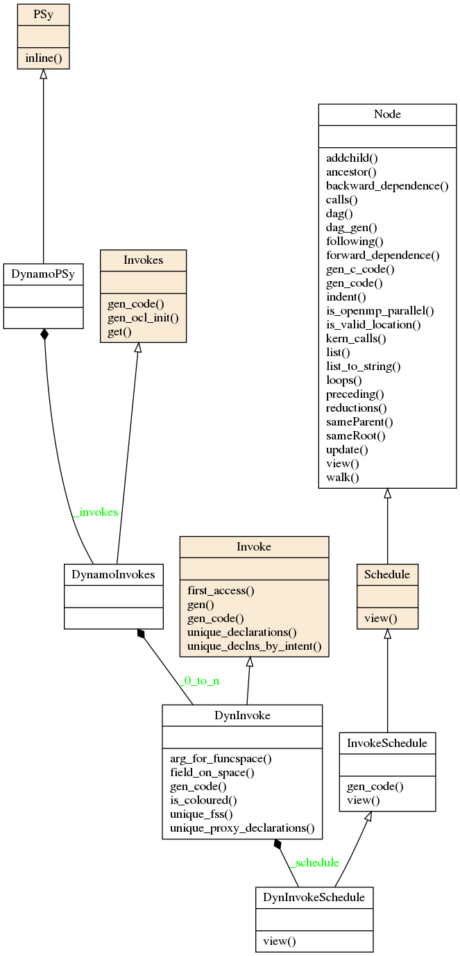
The InvokeSchedule can currently contain nodes of type: Loop, Kernel, Built-in (see the Built-ins section), Directive (of various types), HaloExchange, or GlobalSum (the latter two are only used if distributed memory is supported and is switched on; see the Distributed Memory section). The order of the tree (depth first) indicates the order of the associated Fortran code.

PSyclone will initially create a “vanilla” (functionally correct but not optimised) InvokeSchedule. This “vanilla” InvokeSchedule can be modified by changing the objects within it. For example, the order that two Kernel calls appear in the generated code can be changed by changing their order in the tree. The ability to modify this high level view of a InvokeSchedule allows the PSy layer to be optimised for a particular architecture (by applying optimisations such as blocking, loop merging, inlining, OpenMP parallelisation etc.). The tree could be manipulated directly, however, to simplify optimisation, a set of transformations are supplied. These transformations are discussed in the next section.

InvokeSchedule visualisation

PSyclone supports visualising an InvokeSchedule (or any other PSyIR node) in two ways. First the view() method outputs textual information about the contents of a PSyIR node. If we were to look at the LFRic eg6 example we would see the following output:

>>> print(schedule.view())
InvokeSchedule[invoke='invoke_0', dm=True]
    0: Directive[OMP parallel do]
        Schedule[]
            0: Loop[type='dofs',field_space='any_space_1',it_space='dofs','upper_bound='ndofs']
                Literal[value:'NOT_INITIALISED']
                Literal[value:'NOT_INITIALISED']
                Literal[value:'1']
                Schedule[]
                    0: BuiltIn setval_X_code(p,z)
                    1: BuiltIn X_innerproduct_Y_code(rs_old,res,z)
    1: GlobalSum[scalar='rs_old']

The above output tells us that the invoke name for the InvokeSchedule we are looking at is invoke_0 and that the distributed_memory option has been switched on. Within the InvokeSchedule is an OpenMP parallel directive containing a loop which itself contains two built-in calls. As the latter of the two built-in calls requires a reduction and distributed memory is switched on, PSyclone has added a GlobalSum call for the appropriate scalar.

Second, the dag() method (standing for directed acyclic graph), outputs the PSyIR nodes and its data dependencies. By default a file in dot format is output with the name dag and a file in svg format is output with the name dag.svg. The file name can be changed using the file_name optional argument and the output file format can be changed using the file_format optional argument. The file_format value is simply passed on to graphviz so the graphviz documentation should be consulted for valid formats if svg is not required.

>>> schedule.dag(file_name="lovely", file_format="png")

Note

The dag method can be called from any node and will output the dag for that node and all of its children.

If we were to look at the LFRic eg6 example we would see the following image:

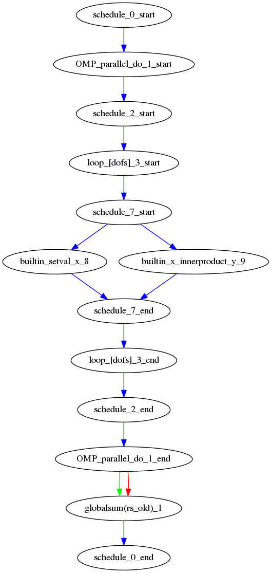
In the image, all PSyIR nodes with children are split into a start vertex and an end vertex (for example the InvokeSchedule node has both schedule_start and schedule_end vertices). Blue arrows indicate that there is a parent to child relationship (from a start node) or a child to parent relationship (to an end node). Green arrows indicate that a Node depends on another Node later in the schedule (which we call a forward dependence). Therefore the OMP parallel loop must complete before the globalsum is performed. Red arrows indicate that a Node depends on another Node that is earlier in the schedule (which we call a backward dependence). However the direction of the red arrows are reversed to improve the flow of the dag layout. In this example the forward and backward dependence is the same, however this is not always the case. The two built-ins do not depend on each other, so they have no associated green or red arrows.

The dependence graph output gives an indication of whether nodes can be moved within the InvokeSchedule. In this case it is valid to run the built-ins in either order. The underlying dependence analysis used to create this graph is used to determine whether a transformation of a Schedule is valid from the perspective of data dependencies.